Mathematical models are predominantly used in science, especially in the natural sciences. Classic areas of application here are theoretical physics or, currently very prominent, epidemiology. But also, and here of course particularly closely thematically connected, in the field of operational research, with all the questions of corporate planning and logistics.
Table of contents
About mathematical models and real problems
A small example to get to know – Bruno Banks beer bench sets
Sources
Author
About mathematical models and real problems
At first glance, mathematics and its theoretical models may have little in common with the real world. Already at school, in the rarely popular subject of mathematics, the question is often asked: Why do we need that? But if you take a second look, you will realise that mathematical models lie behind many everyday processes and real questions. Just where? For example: The students’ gnawing thoughts about finding the shortest path between the stations of the pub crawl. The efforts of the young restaurateur to come up with an ideal menu pricing. Determining the optimal quantities of food and drinks for the summer party. How can the entrepreneur Bruno Bank meet the conditions of his backer? But more on that later. All these questions can be described by means of mathematical models and consequently calculated and solved with mathematical methods.
Of course, mathematical models are mainly used in science, especially in the natural sciences. Quite classically and since time immemorial in theoretical physics, which explains physical processes with its mathematical models. Among others, also in epidemiology, which has recently moved into the limelight and describes the spread of viruses with suitable models. But also, and here of course particularly closely thematically connected, in the field of operational research, with all the questions of corporate planning and logistics.
But what can be understood by a mathematical model? A mathematical model can be seen as a set of mathematical functions, rules, equations and inequalities that in their entirety describe a real problem in the language of mathematics. The model should be computable, so that it can be calculated and solved with mathematical tools. Unfortunately, there is no generally valid recipe for modelling, i.e. the step from the real problem to the model. However, a few basic guidelines can help. What is essential, what can be dispensed with? It is important to model only those aspects that are really relevant to the process. As a rule, a model is always a simplification of the real initial situation. How accurate do the answers need to be? It is also worth thinking about the scales and units used (e.g. place and time). Using appropriate scales helps to keep the model at a predictable meaningful size. And last but not least, what are the goals to be achieved? It is often not obvious to derive a clear objective from a real-world question, but this is essential for a good model.
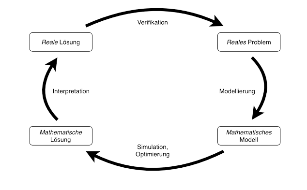
The art of mathematical modelling is to create a model that is as simple as possible and describes the real problem as well as possible. The modelling process is not a fixed sequence of sequential steps. There is no fixed procedure, no recipe that will always lead to success. Rather, the modelling process can be schematically understood as a cycle, the steps of which usually have to be gone through several times.
A small example to get to know – Bruno Banks beer bench sets
Bruno Bank has launched a small start-up company. He wants to produce and sell innovative beer bench sets. However, he does not have his own workshop and has to rent it for €1000 per month for the production of his sets, regardless of how many sets are produced. The production of one set costs Bruno 25 €. The production of one set per month would therefore cost Bruno, for example, 1025 € and of 100 sets 3500 €. However, Bruno cannot produce more than 500 sets per month because he works alone. A warehouse is available for the clothings produced, with storage costs averaging €2 per clothings per month. The finished clothings can be stacked well, so it can be assumed that there is unlimited storage space. Bruno has already produced 10 sets and they are stored in the warehouse.
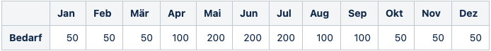
From enquiries already made and demand analyses, Bruno was able to create projected monthly sales figures, which show the greatest values in the summer:
Table 1: Demand forecast for beer bench sets for the coming year
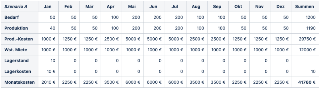
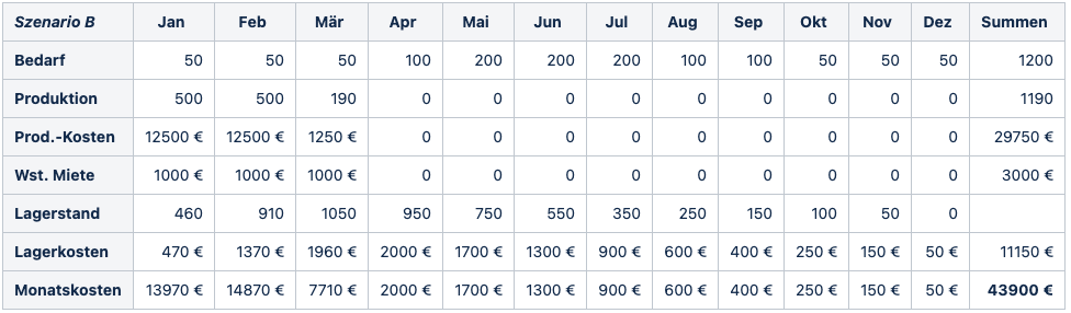
Bruno Bank has been able to win over investor Gabi Geld as a backer for his idea with the beer benches, who will support him with € 37,000. However, she places a condition on his business planning. The production has to be coordinated with the demand forecast and the resulting production costs have to be covered by the money provided. But how is he supposed to achieve this? Bruno decides to set up a few production scenarios and calculate their costs. Maybe he can find a minimum-cost production. Two scenarios seem particularly promising to him. One is to produce exactly the forecast quantity per month (scenario A) so as not to need the warehouse. The other time, the entire annual demand quantity is to be produced right at the beginning of the year (scenario B), so that the workshop is then no longer needed. Bruno calculates the expected costs for both production scenarios and receives 41760 € for scenario A and 43900 € for scenario B. The costs are calculated from the monthly costs of the workshop. Where the costs result from monthly storage, workshop rent and production. It was immediately clear to Bruno how to calculate the costs of workshop rent and production. For the storage costs, he finally assumes that the stored quantity changes evenly from the level at the beginning of the month to the level at the end of the month (linear progression).
Table 2: Calculated costs for scenario A (minimum warehouse use)Table 3: Calculated costs for scenario B (minimum workshop use)
The first production scenario A already seems to be quite good, but its investor Gabi Geld still finds the planned production too cost-intensive. But are there still significantly more cost-effective options? To be really sure, he asks his old school friend and mathematician, Otto Optimal, for help.
Otto Optimal is enthusiastic about Bruno’s beer benches as well as his production planning problem and will support his old friend with his knowledge of optimisation problems. He is also to receive one of Bruno’s trimmings in return. To solve Bruno’s production problem, Otto will first create a mathematical model of the problem, which he will then solve with a suitable solution algorithm for optimality. In this way, the optimal solution, or the optimal production scenario, will be found without a doubt.
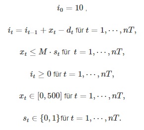
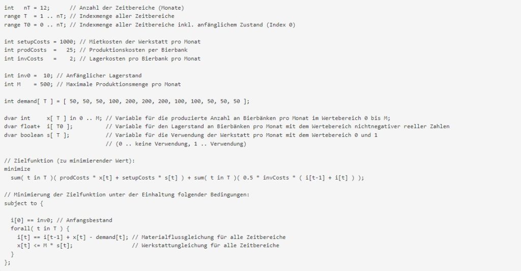
As a first step in modelling, Otto considers variables for the model. The ideal monthly production quantities of the sets are sought. Thus there are 12 time periods (nT = 12) and one product type (beer bench set). The production quantity per month is to be described by the variable t ∈ [ 0 , 500 ] for t = 1, … nT, since the production is limited to 500 pieces per month. Furthermore, it ≥ 0 will describe the stock level (i0 = 10 for the initial stock level) and st the use of the workshop per month (0 … no use, 1 … use). But how should these variables behave now? Necessary constraints will subsequently determine the interaction of the variables. As a second step of the modelling Otto identifies two such constraints: the material flow equation, which describes the stock levels and their outflows and inflows per month, and the workshop equation, which describes the use of the workshop. The stock level it in month t can be characterised by the stock level of the previous month it-1 by the production xt and the demand dt of the current month t:
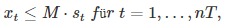
The use of the workshop is necessary as soon as at least one set is produced. This property is described by the following inequality:
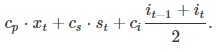
where M stands for an upper bound for the range of values of xt ∈ [ 0 , 500 ] (maximum production quantity per month), which in this case is given by 500. As a last step, Otto describes the costs of production by means of a cost function (or an objective function). The costs incurred are divided into costs for production, storage and workshop and are represented by the coefficients cp, ci and cs (cp = 25, ci = 2, cs = 500 ). The costs per month t can thus be described as follows:
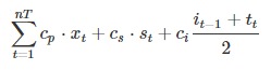
Otto can now formulate the entire optimisation model. The objective is to minimise the objective function while complying with the constraints by optimally choosing the variables:
Minimise the objective function
subject to compliance with the ancillary conditions listed
Whereby the occurring variables have the following meaning:
Variable
Meaning
it
Stock level per week t
xt
Workshop use per week t
st
Production quantity per week t
On closer inspection Otto notices that all occurring functions and equations are linear in the variables, which are themselves binary (discrete) (st) or continuous (it, xt). Such a model is called a mixed integer (linear) model (mixed integer (linear) program … MI(L)P). The present model is a simplified variant of the Capacitated Lot-Sizing Problem (CLSP) known in the literature, which falls into the field of dynamic lot-sizing.
Otto now solves this optimisation model with an MIP solution tool available to him, which implements a branch-and-bound or branch-and-cut algorithm. To do this, he writes his mathematical model in a modelling language so that the solution tool can read the model and then solve it.
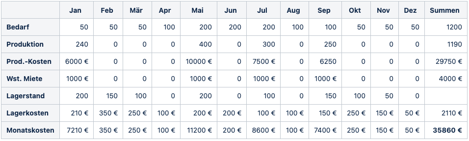
As expected, the optimal objective function value of 35860 € undercuts the values of Bruno’s two production scenarios, even by about 15 %. But in particular, the optimal production scenario clearly fulfils the requirement of the investor Gabi Geld.
Table 4: Optimal production scenario
The next day, Otto proudly presents Bruno with the optimal solution (as in Table 4). Bruno can now fulfil Gabi Geld’s condition and present a sufficiently cost-effective and even cost-optimal planning of the beer bench production.
Finally, Bruno, Gabi and Otto meet for an exchange about further cooperation. Naturally, they enjoy a cool beer on one of Bruno’s sets, much to their benefit.
Sources
H. Paul Williams, Model Building in Mathematical Programming, 5th edition, 2013, John Wiley & Sons Ltd.
Laurence A. Wolsey, Integer Programming, 1998, John Wiley & Sons Inc.
Yves Pochet, Laurence A. Wolsey, Production Planning by Mixed Integer Programming, 2006, Springer Science+Business Media, Inc.
George L. Nemhauser, Laurence A. Wolsey, Integer and Combinatorial Optimization, 1999, John Wiley & Sons Inc.